A* Path Planning Algorithm

 

The A* path planning algorithm is a popular search algorithm used in robotics for identifying the most efficient path from one point to another, avoiding obstacles and adhering to defined constraints along the route.  This algorithm can guarantee the shortest travel path between two points and identifies the optimal path without performing any unnecessary exploration of the map.  The algorithm for identifying an efficient path between two points is, in itself, efficient.

 

I will outline how this algorithm is designed and how it identifies the most optimal path by efficiently exploring a map and calculating the cost of pursuing various routes between two defined points: origin and destination.  I’ve also written and published my own A* algorithm code to demo for various maps with and without obstacles!

 

The cost functions defining a node’s score are measured as distances, and some distance measurements serve specific purposes.  Two of the most popular distance calculations are:

·         Euclidean Distance: Measures straight-line distance between two points.  Allows diagonal movements.

 

·         Manhattan Distance: Measures distance along grid-based movement.  Allows horizontal and vertical steps only.

 

While the two distance methods above are popular, the list is not exhaustive.  After selecting a distance calculation method, we can begin exploring the map and assigning node scores to help identify the most optimal path between two points.  The h(n) heuristic function measures the distance between a node and the destination node.  The g(n) cost function measures the distance between a node and the origin node.  Summing h(n) and g(n) yield the node’s score, f(n), quantifying the cost of an agent traveling to that node.  The f(n) score is the primary metric for assessing the most optimized path for travel

 

 

 

Plan a Path

 

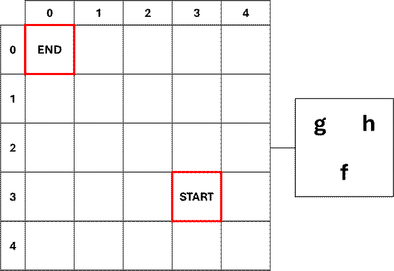
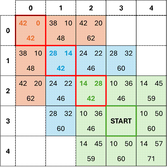
In this example, the map indexes rows and columns from the top left node.  Nodes’ coordinates are presented as (row, col):

·         START: (3, 3)

·         END: (0, 0)

 

Each node displays the h(n) score at the top right, the g(n) score at the top left, and the f(n) score at the bottom.

 

 

Iteration 1

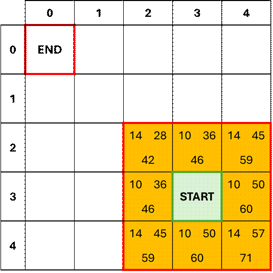
The algorithm starts at the origin node and calculates h(n) and g(n) for each of its immediate neighboring nodes.  The node from which we identify neighboring nodes will be called the ‘focus node’ throughout this post.  We will be using the Euclidean distance to score each node since we want to allow for diagonal movements along the map. 

Once these two metrics are calculated, they’re summed for each neighbor node to define its cost score, f(n).

 

 

As we iterate through the nodes, it’s important that we keep track of focus nodes so we don’t explore them again to eliminate exploration redundancy (i.e. not score a node and its neighbors more than once).  These focus nodes will enter a ‘closed’ state, meaning future iterations can’t access them as focus nodes for exploration anymore.  Scored neighbors remain in an ‘open’ state, meaning they can be selected as future focus nodes.  Unscored nodes cannot be selected as focus nodes until they have been scored from a focus node.

At this point we have one ‘closed’ node and 8 scored ‘open’ nodes. These open-state nodes must be sorted in ascending order along the f(n) score, then the h(n) score. Secondarily sorting open nodes along their h(n) score breaks potential ties between nodes that have the same f(n) score.  We choose to secondarily sort along h(n) because it encourages the algorithm to select the open node that’s closest to the destination node.

We can now consider the whole map as we sort all ‘open’ nodes and select the node with the LOWEST score (i.e. global minimum).  In this example, the lowest node score from exploration iteration one is 42, which makes sense since that node is closest to the destination – an indication that we are buidling a path to the destination node!  The node with score 42 now becomes the focus node in the next iteration.

 

 

 

TIP:  Keep a log of what focus node a subsequent focus node comes from.  We will call this a focus node’s ‘parent’ node.  We will use this at the end!

 

 

Iteration 2

Now that we have identified the next iteration’s focus node and logged its parent node, we can proceed to score its immediate neighbors.  Again, we have one focus node and 8 neighbor nodes.  However, this time we have neighbor nodes that were scored in the previous iteration.  How do we handle this?  Easy! 

Calculate the new h(n), g(n), and f(n) scores for all 8 immediate neighbor nodes.  If a neighbor node already has a set of scores from a previous iteration, then we compare the scores to the current iteration scores.  If the f(n) score from the current iteration less than the existing scores, then replace the node’s score with the lower scores.  If f(n) score from the current iteration is greater than the existing scores, then leave the node scores as they are.

This makes sense because we are looking for the ‘cheapest’ cost path between origin and destination.  If a node’s score drops between iterations, then that may mean there was a more efficient rout for arriving at that node.

 

 

 

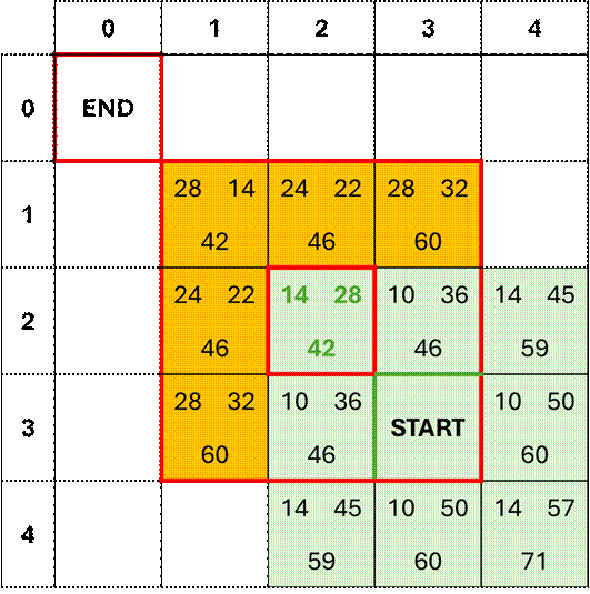
At this point we have two ‘closed’ nodes and 12 open nodes from iterations 1 and 2, as indicated in the figure below.  We have to choose our next focus node by again sorting the open nodes in ascending order along the f(n) score, then the h(n) score and selecting the node with the lowest score.  Again, the lowest open-node score is 42 and that node becomes the focus node for the next iteration in the algorithm.

 

 

 

Iteration 3

For the third iteration, we set the minimum-score node from iteration 2 as the new focus node and score its immediate neighbors.  Again, we calculate the new h(n), g(n), and f(n) scores for all 8 immediate neighbor nodes. 

If a neighbor node already has a set of scores from a previous iteration, then we compare the scores to the current iteration scores.  If the f(n) score from the current iteration less than the existing scores, then replace the node’s score with the lower scores.  If f(n) score from the current iteration is greater than the existing scores, then leave the node scores as they are.

 

 

 

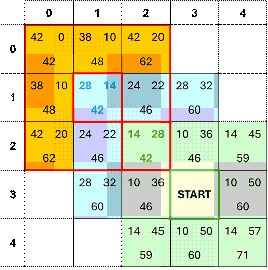
We now have 16 open nodes from iterations 1, 2, and 3 to sort along f(n) then h(n) and determine the next focus node.  Based on the score map above, we identify the open node with f(n) score of 42 as the global minimum, making it the next node for exploration...if there is a next iteration!  Notice that h(n) at this node is 0, and h(n) measures the distance from the current node to the destination node.  Since h(n)=0, this indicates that we have arrived at our destination and do not need to continue exploring nodes.

 

 

Algorithm complete!

 

 

 

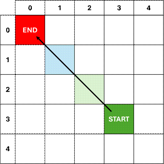
Plan a Path with an Obstacle

 

This next example will follow the same steps in the previous example, but now the agent will navigate around a known obstacle in the map.

 

 

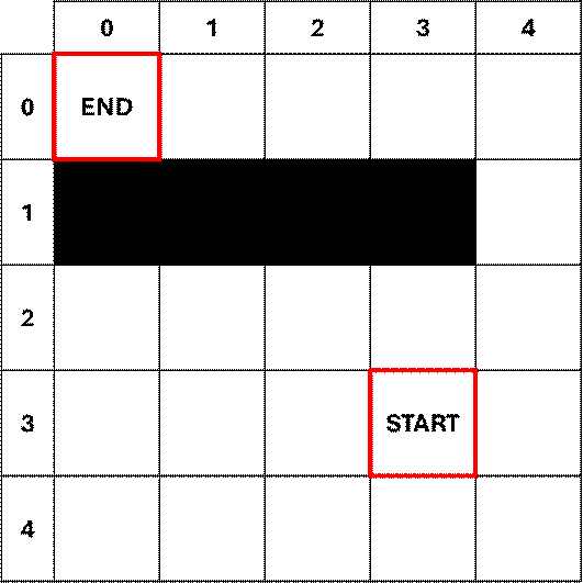
The algorithm from the previous example holds true in this obstacle example.  Nodes that have an obstacle are inaccessible, and so they remain unscored for the duration of path planning.  By leaving the obstacle nodes unscored, they’re omitted from the iterative selection of focus nodes, so they are never selected as potential path nodes.

 

Below is a complete table of focus nodes and parent nodes in the order that they were identified by the algorithm for the obstacle map.  The map is comprised of 25 nodes, of which 21 are accessible.  18 Focus nodes were explored but traversing all 18 to arrive at the destination node is not the most efficient path from the origin node.

 

 

Remember when I advised tracking each focus node’s parent node?  This is where we use that!

 

Starting with the destination node (this should be the last focus node logged chronologically), take the parent node and make that the next focus node.  Check this new focus node’s parent node and make it the next focus node.  Continue this iterative process until you’ve worked your way backwards to the origin node and that will reveal the most optimized path between the origin node and the destination node.

 

 

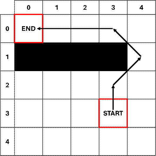
Plotting the optimized path focus nodes confirms that we have selected a viable.

 

Algorithm complete!

 

 

Helpful Resources

• A* Path Finding
• Path Planning Basics
• A* Search Algorithm - Computerphile